Monte Carlo Simulations for FIRE: Better Than Backtesting?

Monte Carlo simulations

Monte Carlo simulations may sound fancy, but they are actually a very simple technique. Indeed, Monte Carlo consists of generating many scenarios. Each of these scenarios is generated using a normal distribution (also called a Gaussian distribution). The distributions are based on the mean and standard deviation of the historical data.

So, to do a Monte Carlo simulation for FIRE, we need to compute the mean and standard deviation for each asset, inflation, and potentially exchange rates. Then, we can run a number of simulations where we generate new returns and inflation for each month. Typically, we would run 10,000 simulations.

Since we want to apply this to Financial Independence and Retire Early (FIRE), we will apply this to our historical dataset of stocks and inflation.

FIRE simulations

Over time, on this blog, I have done many FIRE simulations. I am using my own complete tool to do historical simulations for FIRE. This tool is what I use to refresh the results of the Trinity Study. For these simulations, I have added support for Monte Carlo simulations into my tool.

So, for FIRE simulations, instead of using monthly data, we use Monte Carlo to generate a monthly return, inflation, and exchange rate, and the system remains entirely the same. We can still do rebalancing, fees, glidepaths and all these features.

I will base my Monte Carlo simulations on data from the stock market from 1871 to 2025. I will also be using the inflation in the United States from the same period.

In these simulations, I will do yearly rebalancing and will assume fees of 0.10%.

For these results, I am using 10,000 simulations for each test. Monte Carlo is random, so each result can be different, but with 10,000 simulations, you get a good average. It is worth mentioning that I am using a distribution for inflation and another distribution for stocks. This means that I am doing uncorrelated Monte Carlo distributions. In theory, there is a correlation between stocks and inflation. So I could use a bivariate distribution to model this, but I did not go this far.

I will compare the results of Monte Carlo simulations with two other techniques:

• Pure historical simulations (backtesting)
• A technique that reorders the past (bootstrapping)

Backtesting is the most standard technique, where we run a test on a strategy on historical data. Bootstrapping creates multiple pasts based on historical data by shuffling years around. By comparison, Monte Carlo simulations are creating futures based on historical averages.

If you would like to learn more about the other two techniques, you should read the article where we compare backtesting and bootstrapping for FIRE.

It is worth repeating that since bootstrapping and Monte Carlo simulations are based on random distributions, we can get weird progressions where a higher withdrawal rate has a higher success rate or higher terminal values than a lower one. With enough simulations, this smooths out, but this phenomenon is normal.

Success rate

Our first test will be to check the success rates with the different methods and different portfolios. We will start with retirement periods of 30 years.

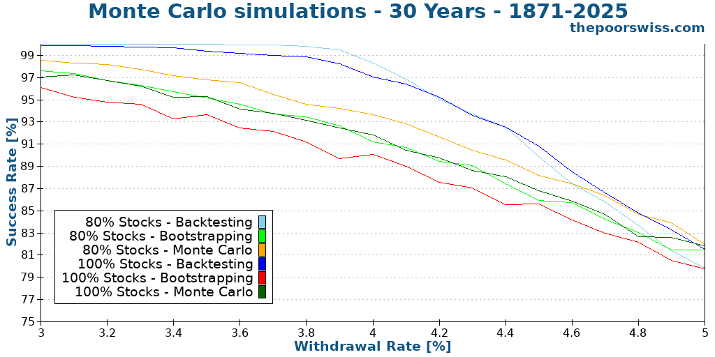
These results are already quite interesting. We can see that the results of Monte Carlo simulations sit between bootstrapping and backtesting. I was expecting Monte Carlo simulations to yield worse results because of the lack of correlation. However, in this case, the lack of correlation plays in our favor. Indeed, it also means we can get higher returns than in history, which can lead to a higher success rate.

The difference with bootstrapping can largely be explained by the lack of correlation between inflation and stocks. Historically, inflation and stock returns have mostly been negatively correlated. With bootstrapping, we get that correlation and end up with high inflation and low returns, worsening the success rate. Since we have not modeled this correlation with Monte Carlo, we end up with better results and avoid some of those years with low returns and high inflation.

If we take the famous 4% withdrawal rate and 100% stocks as an example, we get a difference of 7% between backtesting and bootstrapping but only a difference of about 5% between backtesting and Monte Carlo simulations.

We can also observe that for a high withdrawal rate, the results obtained with Monte Carlo simulations have higher success rates than historical simulations.

We can switch to 40 years of retirement periods to see if the same results are achieved:

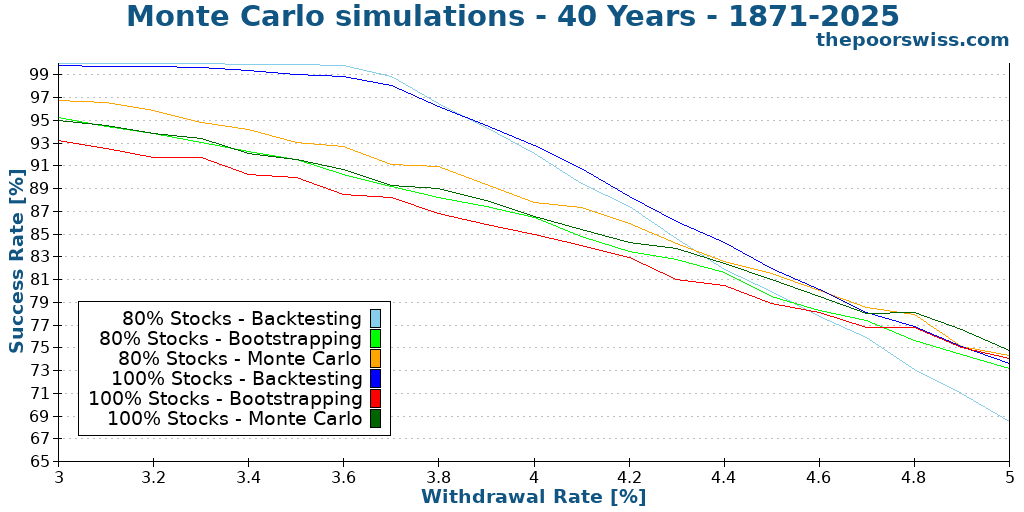
Indeed, we can still observe similar trends. Monte Carlo simulations have lower success rates than backtesting (except at higher withdrawal rates), but they have higher success rates than bootstrapping. We can also see that the differences appear to be smaller between the different methods. Additionally, the point at which Monte Carlo is more successful than historical simulations continues to shift toward lower withdrawal rates—though still at rates that would be unlikely to be sustainable.

We can continue with 50-year retirement periods to see if anything changes:

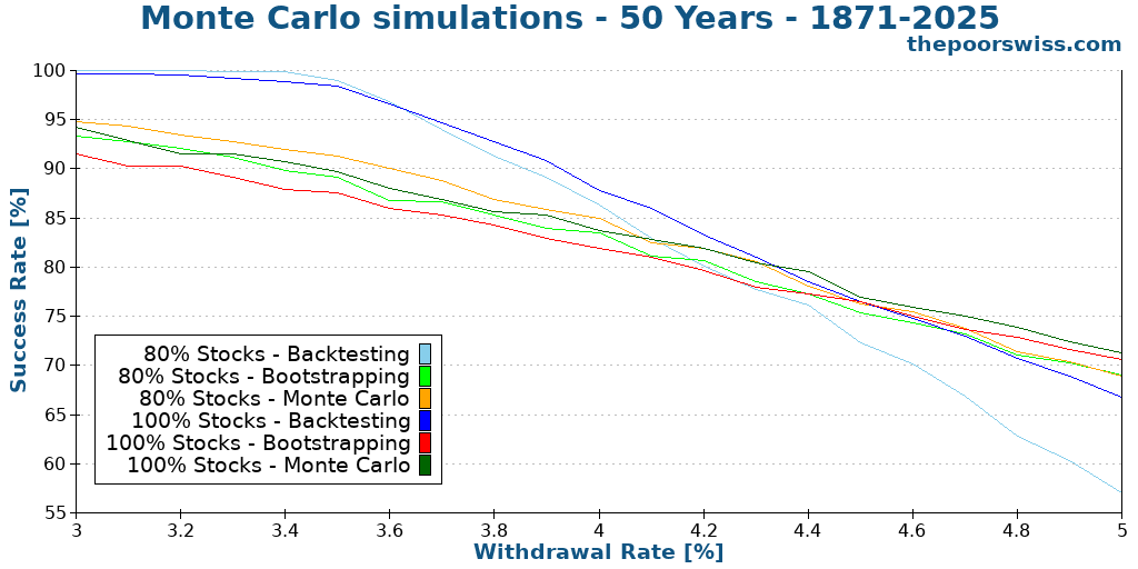
We can see that the trend continues:

• The order of the different methods remains the same.
• The gap between the different methods continues to shrink slowly.
• The point at which the Monte Carlo simulations yield higher success rates than historical simulations continues to shift toward lower withdrawal rates.

Terminal values

A very interesting measure to compare different methods is to look at the terminal values of the simulations. The terminal value is the amount left at the end of the simulation. Any amount above zero would indicate a success. It is interesting to note that average terminal values are usually much higher than we would expect (because averages are skewed towards extremes). But it allows one to quickly visualize differences.

For that, we look at the average terminal values after 40 years with 100% stocks.

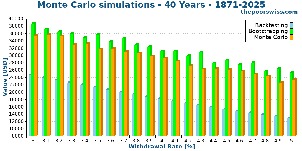
One thing is very interesting to notice: Monte Carlo results are once again between backtesting and bootstrapping. And they are much closer to bootstrapping than they are to backtesting.

When we remove the sequence of returns risk entirely, we observe much higher average terminal values. The reason is that this creates sequences with very long bull markets that have not happened in history. History has cycles with bull markets followed by bear markets. On the other hand, Monte Carlo simulations can create sequences without cycles. We could see better with consistent high returns over 50 years. This cannot happen with backtesting since it has never happened. But it can happen with bootstrapping and Monte Carlo.

We can check whether the same stands for 50 years:

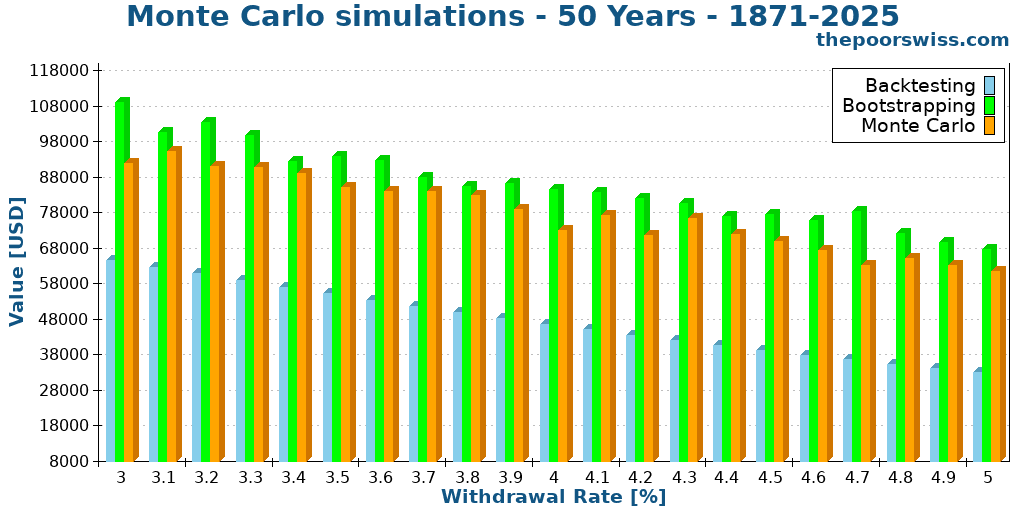
The results are indeed almost similar. The scope of the numbers is increasing, but the difference between the different methods is mostly the same. At high withdrawal rates, we can see that the gap is now smaller but still significant.

Worst duration

I usually finish my analysis with the worst duration metric. This metric shows how early a strategy can fail. For instance, a worst duration of 300 months means that the strategy could have failed after 25 years. Such a number is good if you are simulating for 30 years but terrible if you are simulating for 50 years.

So, we can see what is the worst duration for all these methods.

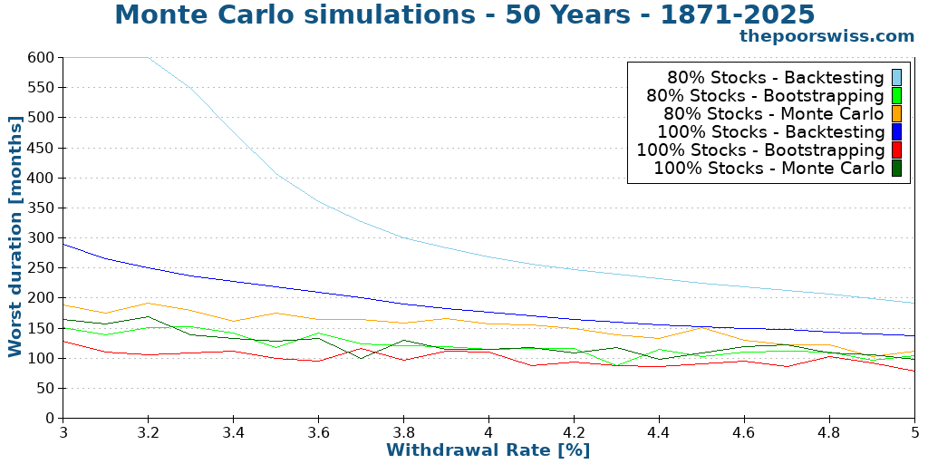
We can observe the same trends as before, where Monte Carlo results sit between backtesting and bootstrapping results. The lack of correlation between years really hurts the worst-case scenario. Indeed, just like the distributions could craft a sequence of excellent years, the distributions could create a sequence of terrible years. This results in a very low worst-case duration.

Shorter periods

Backtesting really needs a lot of data to be accurate. As a result, it cannot yield good results in short periods of time. For instance, you cannot simulate 50 years of retirement based on 40 years of data. Monte Carlo has no issue with that. So, we can simulate results for short periods and see how they compare.

In the previous installment of our series, I tested periods of 50 years. To avoid repeating the same analysis, I have tested Monte Carlo on periods of 25 years to see the differences.

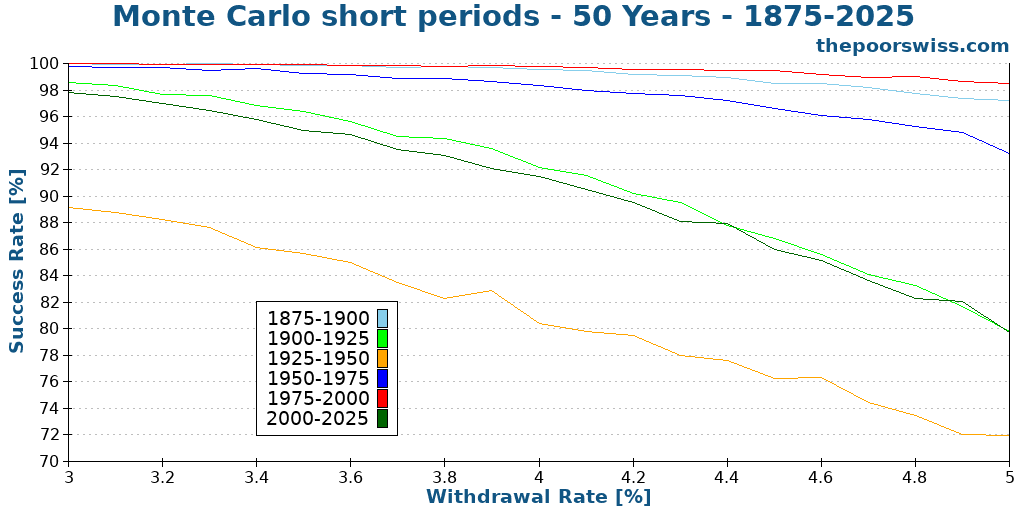
These results are more interesting than I expected! I was innocently thinking that the last 25 years (2000-2025) would be the best period for FIRE, but no. The last 50 years were great, but the last 25 years were only average.

The reason is that 1975-2000 had exceptional returns and below-average crashes. If we compare this to 2000-2025, we had multiple major crashes (the dot-com bubble and the great financial crisis).

On the other hand, it is not surprising to find the 1925-1950 period at the bottom. This period included the Great Depression, the worst time for the stock market in history.

I like these results because they give us a perspective on the difference between different periods in the stock market. Backtesting is incapable of doing that. Other methods can help bridge the gaps. Of course, this does not mean that backtesting is bad, far from it. Backtesting over 150 years of data is quite accurate. However, it is important to realize that different periods in history would have higher or lower success rates.

Try it yourself

If you want to run your own Monte Carlo simulations now, I have a calculator for you. Our advanced FIRE calculator now has a new feature to switch to Monte Carlo simulations (in the form, select Monte Carlo in the simulation method dropdown).

These simulations are currently limited to 2,500 runs to avoid any issues on the servers. This is lower than I used for the simulations in this article (10,000). However, 2,500 simulations should be enough to give reliable results. In the future, I will see whether I can increase it. Requests are cached for performance, so you may not experience too much randomness between multiple runs with the same parameters.

You can also use it directly below by changing the simulation method and comparing the results.

Conclusion

Overall, Monte Carlo simulations offer an interesting method for our FIRE toolbelt. They offer an alternative to the very strict backtesting method. They shine when there is little data since they are much more flexible. And they can simulate periods that have never happened in history.

So, should we skip to only using Monte Carlo simulations? No. Monte Carlo simulations do not replace simulations like backtesting. Since they are not correlated properly, they entirely ignore market cycles. As such, they can generate periods that are not even close to anything that has happened in history.

However, they are a suitable alternative to bootstrapping, which is too pessimistic in my opinion. Using something like Monte Carlo simulations to validate a strategy previously validated only with historical simulations is a good idea. I find that many people are too optimistic with their FIRE withdrawal rate. I find that using such tools can help them. We should not forget that the future is uncertain and that some future periods will be different from what we have known, and this may impact our strategies.

If you would like to explore more simulations, you can try to read our article on finding failsafe withdrawal rates. And please let me know if you would like to find failsafe withdrawal rates with four new Monte Carlo and bootstrapping methods.

What about you? Do you like Monte Carlo simulations? Which simulation method do you use to validate your FIRE strategy?